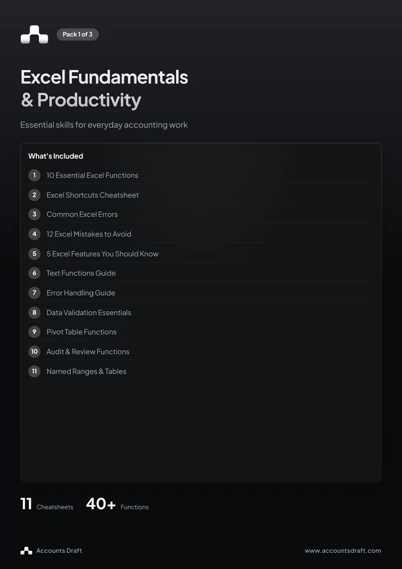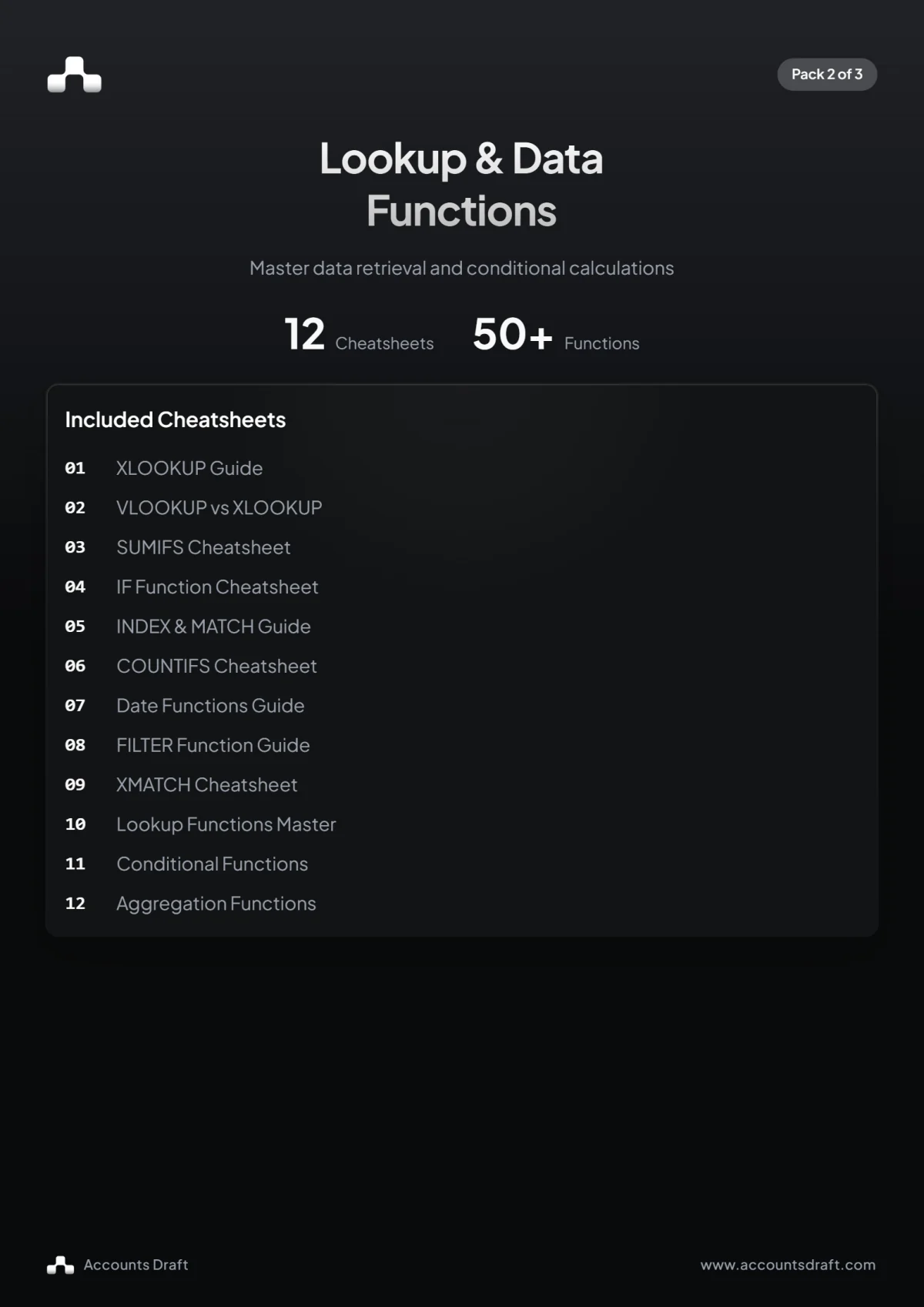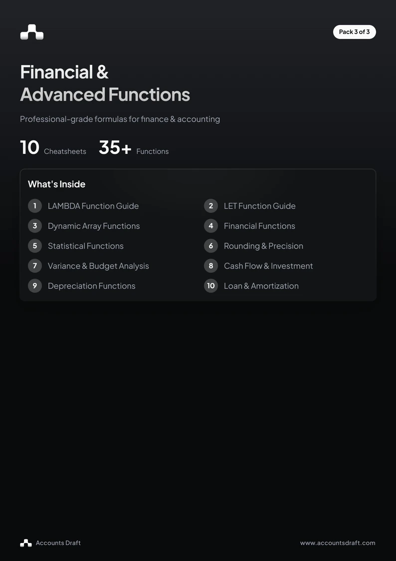
This free Excel financial and advanced functions guide brings together 10 cheatsheets in a 13-page PDF. It covers reusable formulas, dynamic arrays and calculations for financial analysis, with examples for loans, cash flow, budgets and fixed assets.
The guide is labelled Pack 3: Financial & Advanced Functions. Use its contents page to find the topic you need, then keep the relevant cheatsheet beside your workbook.
What is inside the guide?
The first three cheatsheets explain LAMBDA, LET and dynamic array functions, including FILTER, SORT, SORTBY, UNIQUE and SEQUENCE. They show how to create your own functions, name intermediate calculations and return results across several cells.
The remaining pages cover financial functions, statistics, rounding and precision, variance and budget analysis, cash flow and investment analysis, depreciation, and loan amortisation. The financial pages include PMT, IPMT, PPMT, NPV, XNPV, IRR and XIRR.
Make a formula easier to follow with LET
LET gives names to values within a formula. Suppose B2 contains sales and C2 contains costs. This example names the inputs and profit calculation before returning the profit margin:
=LET(sales,B2,cost,C2,profit,sales-cost,profit/sales)With sales of 10,000 and costs of 7,000, the result is 0.3. Format the cell as a percentage to display 30%. Check for zero sales before using this calculation, as dividing by zero returns an error.
The PDF also shows how LET can store a lookup result so the same lookup does not need to be repeated within a formula.
Create a reusable calculation with LAMBDA
LAMBDA lets you define a calculation with named inputs. This example from the guide takes a price and a rate, then applies the rate to the price:
=LAMBDA(price,rate,price*(1+rate))(100,0.2)The result is 120. The final pair of brackets supplies the inputs for this test calculation.
To reuse the calculation, open Formulas, choose Name Manager and create a name such as ADDTAX. Put the following definition in the Refers to field:
=LAMBDA(price,rate,price*(1+rate))You can then call the named function with =ADDTAX(100,0.2). Choose the input rate for your own calculation rather than treating the example rate as a rule.
Build a sorted list with dynamic arrays
The dynamic array cheatsheet combines functions to filter, sort and remove duplicates. If A2:A100 contains the list you want to summarise, use:
=SORT(UNIQUE(A2:A100))UNIQUE returns distinct values and SORT puts them in order. Adjust the range to your actual data and leave clear cells below the formula for the results to spill into.
The guide also introduces TAKE, DROP, VSTACK and HSTACK for selecting or combining arrays. Check that the newer functions you choose are available in your version of Excel, especially when sharing a workbook.
Calculate a monthly loan payment with PMT
PMT calculates a regular payment using a rate, a number of periods and a present value. The guide gives this example for a 25,000 loan over five years at an annual rate of 6%:
=PMT(6%/12,60,-25000)The result is approximately 483.32 per month. The formula divides the annual rate by 12 and uses 60 monthly payments, with payments at the end of each period. The negative loan value produces a positive payment result.
Keep the rate and payment periods consistent. The loan amortisation cheatsheet also covers IPMT for the interest part of a payment, PPMT for the principal part, and cumulative interest and principal functions.
Use NPV or XNPV for cash flow calculations
NPV discounts cash flows at regular intervals. Suppose B2 contains an initial outflow as a negative amount and B3:B7 contains five annual cash flows received at each year end. At a discount rate of 10%, use:
=NPV(10%,B3:B7)+B2The initial outflow is added separately because it occurs at the start, before the future cash flows included in NPV.
For cash flows on specific dates, put their dates in A2:A7 and the corresponding amounts in B2:B7, including the initial outflow. Then use:
=XNPV(10%,B2:B7,A2:A7)Keep each date paired with its amount and use a consistent sign convention for money paid and received. The cash flow cheatsheet also covers IRR, XIRR, MIRR and payback calculations.
Compare actual results with budget
The variance cheatsheet separates the amount of a difference from its percentage. If B2 contains the actual result and C2 contains the budget, the amount variance is:
=B2-C2To calculate the percentage variance while flagging a zero budget for review, use:
=IF(C2=0,"Check budget",(B2-C2)/ABS(C2))Format numeric results as percentages. The absolute budget value keeps the denominator positive, as shown in the guide. Interpret the result in context: higher revenue and higher spending have different implications.
The same cheatsheet includes year-to-date totals, full-year forecasts and run-rate projections. Check the reporting period and consider seasonality when adapting those examples.
Calculate straight-line depreciation with SLN
SLN takes an asset's cost, residual value and useful life. For an asset costing 10,000, with a residual value of 1,000 and a five-year useful life, use:
=SLN(10000,1000,5)The result is annual depreciation of 1,800. The depreciation cheatsheet also covers DB, DDB, VDB and SYD, with examples for fixed asset schedules and book values. Use assumptions that match the asset and the purpose of your calculation.
Check rounding and statistical measures
The rounding cheatsheet covers ROUND, ROUNDUP, ROUNDDOWN, MROUND, CEILING and FLOOR, alongside TRUNC, INT, MOD and QUOTIENT. For example, if B2 contains a price and C2 contains a quantity, round their product to two decimal places with:
=ROUND(B2*C2,2)Changing the cell's number format only changes its display; ROUND changes the calculated value. Decide where rounding belongs and check that any allocated amounts still add up to the original total.
The statistics page brings together averages, medians, standard deviations, ranking, counts and forecasting functions. It distinguishes sample functions such as STDEV.S from population functions such as STDEV.P, helping you choose a measure that matches your dataset.
Keep the PDF as a practical reference
Download the guide and return to the relevant cheatsheet as you work. Adapt the ranges and assumptions to your own workbook, then test formulas against a small set of known results before using them across a report.
The download is a PDF reference guide, with no sign-up required.