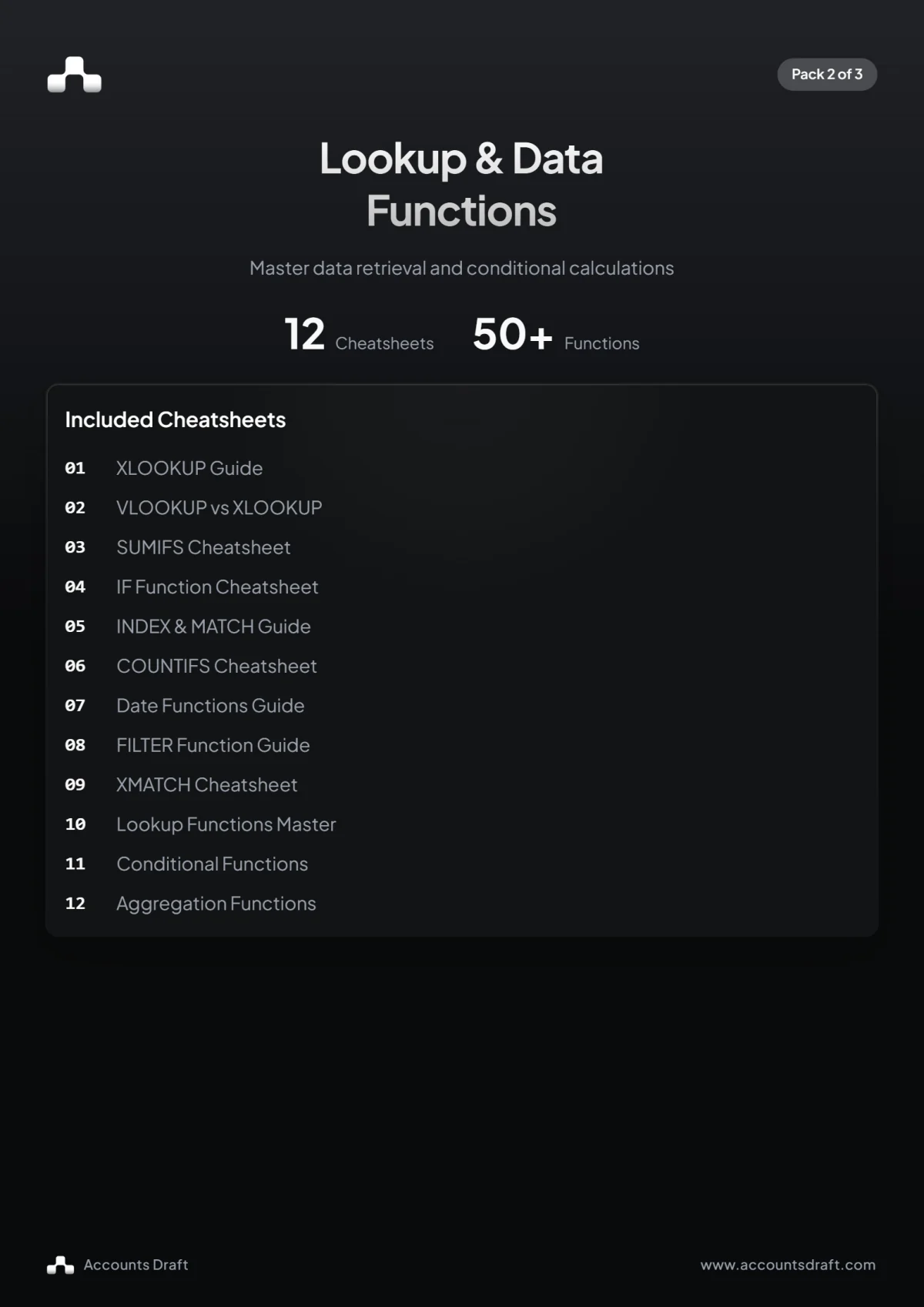
This free Excel lookup and data functions guide brings together 12 cheatsheets in a 15-page PDF. It explains how to find matching records, calculate totals and counts using conditions, work with dates and return filtered results.
The guide is labelled Pack 2: Lookup & Data Functions. Use it as a reference beside your workbook, choosing the page that matches the task you need to complete.
What is inside the guide?
The lookup pages cover XLOOKUP, VLOOKUP versus XLOOKUP, INDEX with MATCH, XMATCH and a wider lookup functions reference. These pages explain function arguments, exact matches, lookup direction and ways to find a value using both a row and a column heading.
The remaining cheatsheets cover SUMIFS, IF, COUNTIFS, date functions, FILTER, conditional functions and aggregation. The aggregation page includes SUMPRODUCT, SUBTOTAL and AGGREGATE, with an example for checking a filtered trial balance.
Find an account name with XLOOKUP
Suppose A2 contains an account code, E2:E100 contains reference codes and F2:F100 contains account names. To return the matching name and show a message when the code is missing, use:
=XLOOKUP(A2,E2:E100,F2:F100,"Not found")XLOOKUP uses an exact match by default. Keep the lookup and return ranges aligned so each code corresponds to the name on the same row. Check that your version of Excel supports XLOOKUP before sharing the workbook.
Use VLOOKUP or INDEX and MATCH in an older workbook
The guide compares XLOOKUP with VLOOKUP and explains where INDEX with MATCH provides another approach. For the same account-code example, VLOOKUP can search the first column of E2:F100 and return the name from its second column:
=VLOOKUP(A2,E2:F100,2,FALSE)FALSE requests an exact match. Omitting it can produce an approximate match, which is unsuitable when you need a specific account code. VLOOKUP searches the first column of its table and returns a value to the right.
INDEX with MATCH separates the return range from the search range:
=INDEX(F2:F100,MATCH(A2,E2:E100,0))MATCH finds the code's position, using 0 for an exact match, and INDEX returns the name at that position. The PDF also shows two-way lookups and explains how XMATCH can search from the end of a range to find the last occurrence.
Total and count records with several conditions
Suppose column A contains client names, column B contains payment statuses and column C contains invoice amounts. To total paid invoices for Example Ltd in rows 2 to 100, use:
=SUMIFS(C2:C100,A2:A100,"Example Ltd",B2:B100,"Paid")SUMIFS starts with the range of amounts to add. Each following range and criterion supplies a condition, and every condition must match for a row to be included.
To count those invoices instead of adding their amounts, use COUNTIFS:
=COUNTIFS(A2:A100,"Example Ltd",B2:B100,"Paid")Keep the ranges the same size and check that amounts are stored as numbers. The cheatsheets also show comparison operators and wildcards for conditions such as values above a threshold or text beginning with a particular word.
Combine IF with AND or OR
IF returns one result when a test is true and another when it is false. AND requires every test to be true; OR requires at least one.
For example, suppose A2 contains an amount and B2 contains a review status. To flag entries above 1,000 that still need checking, use:
=IF(AND(A2>1000,B2="Unchecked"),"Review","")The guide also covers nested IF formulas, IFS and error handling. Choose an error message that helps you investigate missing data rather than hiding a problem behind an unexplained zero.
Calculate month ends with date functions
The date functions cheatsheet covers TODAY, NOW, DATE, EOMONTH, EDATE and NETWORKDAYS, alongside functions for extracting parts of a date.
If A2 contains a date within the reporting month, return that month's final date with:
=EOMONTH(A2,0)Format the result as a date. EDATE moves a date forward or back by a number of months, while NETWORKDAYS calculates working days between dates and accepts a holiday range. Use DATE to construct dates from year, month and day values when regional date formats could be ambiguous.
Return matching rows with FILTER
Using the client, status and amount columns above, FILTER can return every paid invoice for Example Ltd:
=FILTER(A2:C100,(A2:A100="Example Ltd")*(B2:B100="Paid"),"No matching invoices")Multiplying the two conditions requires both to be true. The final argument supplies a message when no rows match. FILTER returns a dynamic array, so leave space for the results to spill into adjacent cells and check that the function is available in your Excel version.
Check totals after filtering a list
The aggregation cheatsheet explains SUBTOTAL function codes and gives a filtered trial balance example. If column D contains debits and column E contains credits, this formula calculates the difference for the visible rows:
=SUBTOTAL(109,D2:D100)-SUBTOTAL(109,E2:E100)Function code 109 adds values while excluding filtered-out and manually hidden rows. Check which rows are visible when interpreting the result; a filtered selection may not balance even when the complete trial balance does.
The same cheatsheet introduces SUMPRODUCT for weighted averages and conditional calculations, and AGGREGATE for calculations with options to ignore errors or hidden rows.
Keep the PDF as a desk reference
Download the PDF and use its contents page to move between the 12 cheatsheets. Adapt the ranges, labels and criteria to your own workbook, then test each formula against a small set of known results before filling it across a report.
The download is a PDF reference guide, with no sign-up required.